1. Introduction: The Architecture of Modern Intelligence
The contemporary landscape of computational intelligence is defined by a rigorous, nested hierarchy of technologies that are frequently conflated in public discourse yet possess distinct architectural and functional characteristics. To navigate the current era of innovation, one must look beyond the marketing vernacular and understand the precise taxonomic relationships between Artificial Intelligence (AI), Machine Learning (ML), and Deep Learning (DL). These terms are not synonyms; rather, they represent a lineage of increasing specialization and architectural complexity, often visualized as a set of Russian Matryoshka dolls where each subsequent technology is entirely contained within the predecessor.1
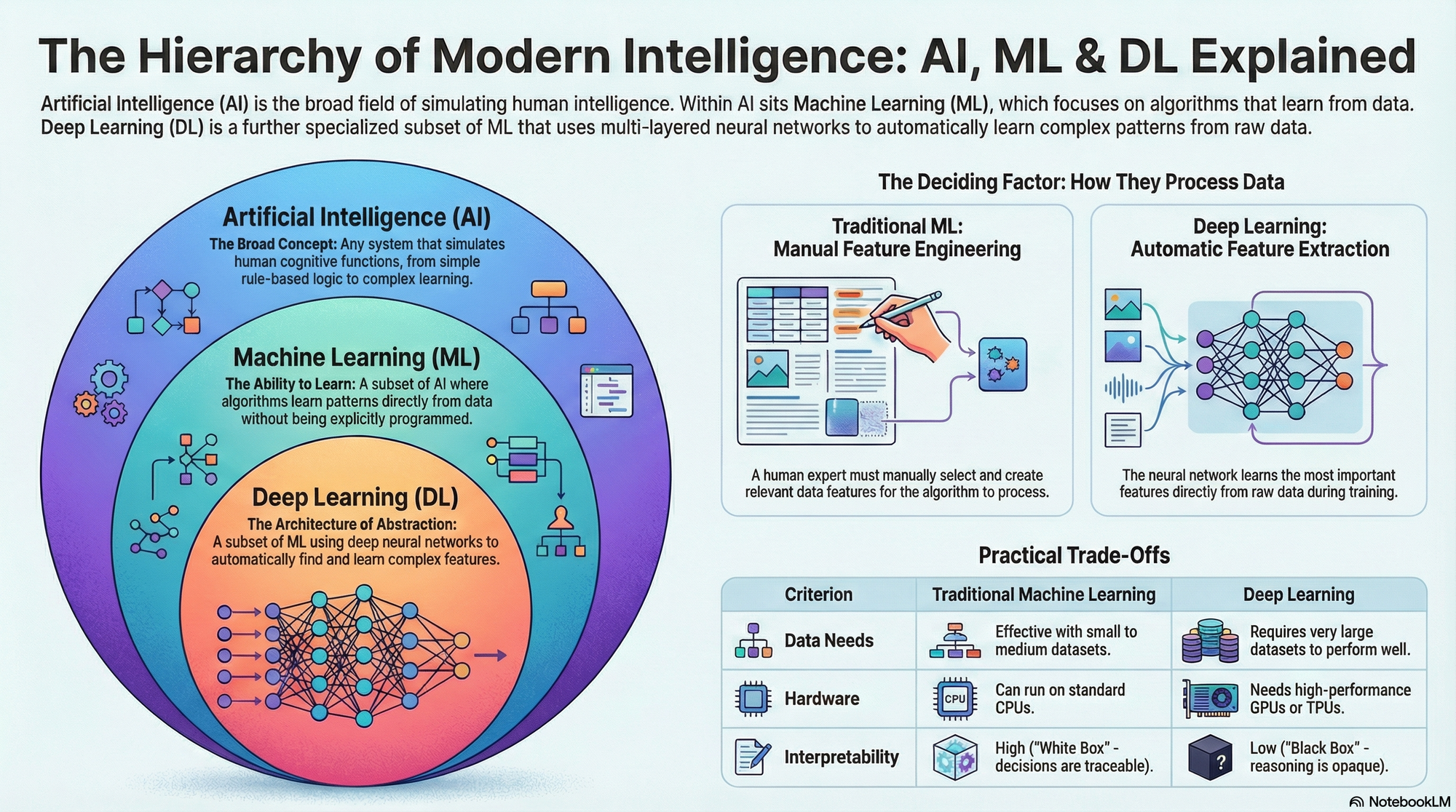
At the highest level of abstraction lies Artificial Intelligence, the broad discipline encompassing any system capable of mimicking human cognitive functions. Within this sphere resides Machine Learning, a subset specifically focused on algorithms that optimize their performance through statistical experience rather than explicit programming. Deep Learning, utilizing multi-layered Artificial Neural Networks (ANNs), constitutes a specialized subset of ML capable of automatic feature extraction and high-level abstraction.3 This report provides an exhaustive deconstruction of this hierarchy, analyzing the technical delineations between ML and DL, the pivotal role of feature engineering versus representation learning, and the three core learning paradigms—Supervised, Unsupervised, and Reinforcement Learning—that drive these systems.
The distinction between these layers is not merely academic; it dictates the operational requirements, hardware infrastructure, and strategic viability of intelligent systems in production. While traditional Machine Learning remains a cornerstone of structured data analytics, Deep Learning has emerged as the requisite engine for processing the unstructured chaos of the real world—images, sound, and natural language. Understanding the "Why" and "How" of this transition requires a deep dive into the mechanics of features, the architecture of neural layers, and the fundamental shift from human-guided optimization to autonomous representation learning.
Slides


Module Explainer Video
2. The Nested Hierarchy: From Logic to Learning
The most accurate conceptual model for these technologies is a concentric hierarchy. There is no intersection where Deep Learning exists outside of Machine Learning, nor where Machine Learning exists outside of Artificial Intelligence. This containment implies inheritance: Deep Learning inherits the statistical optimization principles of Machine Learning, which in turn inherits the goal-directed behavior of Artificial Intelligence.3
2.1 Artificial Intelligence: The Macro-Cosm
Artificial Intelligence serves as the overarching "outer shell" of this hierarchy.1 Historically, this field encompasses a wide array of techniques, ranging from the logic-based, symbolic AI of the 1970s and 1980s to the statistical learning methods that dominate today. The core definition of AI rests on the simulation of human intelligence processes by machines, particularly computer systems. These processes include learning (the acquisition of information and rules for using the information), reasoning (using rules to reach approximate or definite conclusions), and self-correction.3
In the early decades of the field, AI was predominantly "Rule-Based." Systems were designed by human experts who explicitly programmed logic statements—massive trees of "if-then-else" instructions—to handle decision-making. These systems, often referred to as "Good Old-Fashioned AI" (GOFAI), were rigid. They did not "learn" in the modern sense; they executed pre-defined instructions derived from human knowledge.1 For example, a rule-based system for medical diagnosis might rely on a hard-coded rule: "IF temperature > 100 AND patient reports cough, THEN classify as flu." While effective for closed, well-defined environments, these systems were brittle. They collapsed when faced with ambiguity, nuance, or unstructured data that had not been explicitly anticipated by the programmer.1
2.2 Machine Learning: The Paradigm Shift
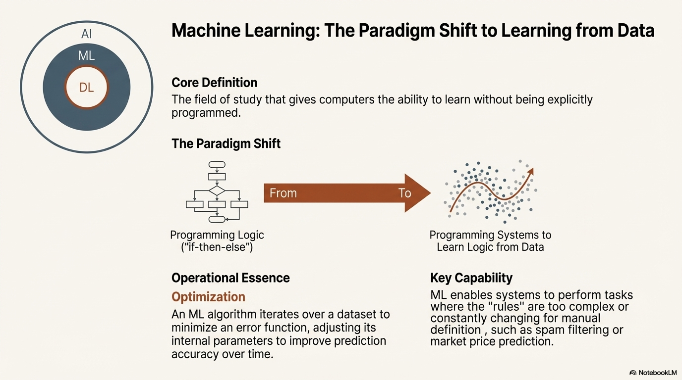
Machine Learning represents the first major contraction and deepening of the field. It marks a fundamental paradigm shift from "programming logic" to "programming systems to learn logic".1 Instead of writing the rules, the engineer writes an algorithm that can derive the rules from data.
ML is defined as the field of study that gives computers the ability to learn without being explicitly programmed.3 It utilizes algorithms and statistical models to analyze data, identify patterns, and make decisions with minimal human intervention.7 The operational essence of ML is optimization. An ML algorithm iterates over a dataset to minimize an error function, adjusting its internal parameters to improve prediction accuracy over time. This capability allows ML systems to perform tasks—such as spam filtering or price prediction—that would be impossible to hard-code using static rules because the "rules" of spam or market dynamics are constantly changing and too complex for manual definition.6
2.3 Deep Learning: The Architecture of Abstraction
Deep Learning is a specialized subset of Machine Learning.3 It is distinguished not merely by its complexity but by its architectural inspiration: the biological neural networks of the human brain.2 The "deep" in Deep Learning refers specifically to the depth of the neural network layers. While a traditional artificial neural network might contain a single hidden layer, Deep Learning algorithms employ multi-layered architectures to model complex patterns in data.8
This layering is not arbitrary. It facilitates a process known as Hierarchical Representation Learning. DL systems process data through successive layers of neurons, where each layer extracts features of increasing complexity. The first layer might detect simple edges in an image; the second combines those edges into shapes; the third assembles shapes into objects. This hierarchical capability allows DL to excel at tasks involving unstructured data, such as image recognition and natural language processing, where traditional ML often struggles due to the difficulty of manually defining relevant features.10
3. Machine Learning (ML): The Foundation of Data-Driven Logic
To understand the necessity of Deep Learning, one must first master the mechanics—and the limitations—of traditional Machine Learning. While powerful, traditional ML is bound by a significant bottleneck: its reliance on human domain expertise for feature engineering.
3.1 The Mechanics of "Shallow" Learning
Traditional ML algorithms, often retroactively termed "shallow learning" to contrast with DL, rely on statistical rigor and mathematical optimization. Common algorithms in this category include Linear Regression, Logistic Regression, Support Vector Machines (SVM), Decision Trees, and Random Forests.11 These methods are often grounded in established statistical theories. For instance, regression models predict continuous numerical values (e.g., house prices) by finding the optimal linear relationship between input variables.13
A defining characteristic of many traditional ML models is their relative transparency or interpretability. In a Decision Tree, for example, the path from input to decision can be traced node by node (e.g., "The loan was denied because income < $50k AND debt > $10k"). This contrasts sharply with the opaque, "black box" nature of Deep Learning networks, where decisions result from the aggregate activation of millions of parameters.5This interpretability makes traditional ML the preferred choice in regulated industries where explaining the "why" behind a decision is as important as the decision itself.
3.2 The Critical Bottleneck: Feature Engineering
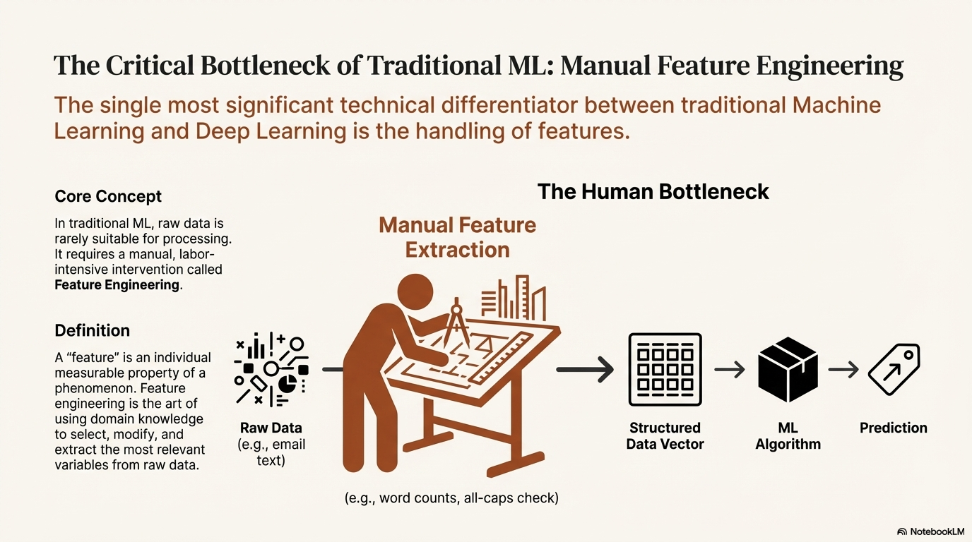
The single most significant technical differentiator between traditional Machine Learning and Deep Learning is the handling of features. In the context of data science, a "feature" is an individual measurable property or characteristic of a phenomenon being observed.14 In traditional ML, the raw data is rarely suitable for immediate processing; it requires a manual, labor-intensive intervention known as Feature Engineering.
3.2.1 The Manual Engineering Process
Feature engineering is the art of using domain knowledge to select, modify, and extract the most relevant variables from raw data to make the ML algorithm work.11 It is a process of translation: converting the messy reality of the world into a structured vector of numbers that a statistical model can digest.
Consider a spam detection system. A raw email is a string of unstructured text. A traditional ML algorithm like Naive Bayes or Logistic Regression cannot "read" the text in the human sense. A human engineer must intervene to define features that might indicate spam. They might create a variable counting the frequency of the word "free," a boolean variable checking for the presence of all-caps in the subject line, or a metric for the ratio of images to text.11 These features are then fed into the algorithm. The algorithm's success is entirely dependent on the engineer's ability to identify which features matter. If the engineer fails to include a feature checking for a specific phishing URL pattern, the model will fail to detect it, regardless of the mathematical sophistication of the classification algorithm.10
This process serves a dual purpose: it extracts signal from noise and reduces the dimensionality of the data. Feature selection is a form of dimensionality reduction, selecting a subset of variables to create a new model that reduces multicollinearity and maximizes generalization.14 By focusing only on the most significant inputs, feature engineering attempts to avoid the "curse of dimensionality," where the volume of data required to statistically model a problem grows exponentially with the number of input variables.15
3.2.2 The Limits of Human Curation
While effective for structured data (like spreadsheets of customer demographics), manual feature engineering breaks down when dealing with high-dimensional, unstructured data like images, audio, or video.
In image analysis, the limitations become glaring. A single 1080p image contains over 2 million pixels, each with Red, Green, and Blue values. The raw input is a massive grid of numbers. Manually defining features for "a cat" in terms of pixel relationships is nearly impossible. How does one mathematically define the curve of an ear or the texture of fur across thousands of variations in lighting, angle, and occlusion?.7
Historical approaches used techniques like Gabor filters, which are mathematical tools used to detect textures and edges by analyzing frequency and orientation. However, these filters required complex parameter adjustments. An engineer would have to manually tune the wavelength and orientation of the filters to detect specific textures. This manual tuning is brittle; a filter tuned to detect a vertical edge might miss a diagonal one, or one tuned for a specific lighting condition might fail in a shadow.10 The result is a system that is difficult to scale and prone to error, as the feature extraction pipeline becomes a complex web of hand-crafted rules that cannot generalize to new, unseen variations of the data.16
3.3 Operational Characteristics of Traditional ML
Despite the bottleneck of feature engineering, traditional ML remains highly effective for specific classes of problems.
- Data Volume: Traditional ML algorithms generally perform well with small to medium-sized datasets. Because the features are hand-curated and theoretically high-signal, the model requires fewer examples to converge on a solution.5
- Hardware: These algorithms are computationally less intensive than Deep Learning. They can often run on standard CPUs and do not require specialized hardware like GPUs or TPUs. This makes them accessible for edge devices or environments with limited compute resources.5
- Training Time: Due to simpler architectures and lower computational demands, traditional ML models can be trained relatively quickly—often in seconds or minutes—allowing for rapid iteration cycles.5
4. Deep Learning (DL) and Neural Networks (NN)
Deep Learning represents the evolutionary leap designed to overcome the limitations of manual feature engineering. By utilizing Artificial Neural Networks (ANNs) with multiple hidden layers, DL systems introduce the capability of Automatic Feature Extraction, also known as Representation Learning. This shift moves the burden of feature identification from the human engineer to the mathematical architecture of the network itself.
4.1 The Artificial Neural Network (ANN)
At the core of Deep Learning lies the Neural Network. While modern ANNs are mathematical constructs rather than biological simulations, they draw conceptual inspiration from the human brain's architecture of neurons and synapses.2
4.1.1 The Anatomy of a Node
The fundamental unit of an ANN is the neuron, or node. Its operation is a mathematical abstraction of a biological neuron's firing mechanism. A node receives input data, applies a weight to each input, adds a bias, and passes the result through an activation function.17
- Weights: These represent the strength of the connection between neurons. During training, the network adjusts these weights to increase or decrease the influence of specific inputs. A high weight implies that the input is significant for the desired output.17
- Biases: The bias allows the activation function to be shifted to the left or right, effectively setting a threshold for when the neuron should be activated.
- Activation Function: This is the critical component that introduces non-linearity to the system. Without activation functions, a neural network, no matter how many layers it has, would behave like a single linear regression model. Functions like ReLU (Rectified Linear Unit) or Sigmoid determine whether a neuron "fires" (passes data to the next layer). This non-linearity allows the network to learn complex, curved boundaries between data classes rather than just straight lines.18
4.1.2 The Structure of Layers
The distinction between a simple Neural Network and "Deep Learning" is structural. A basic neural network consists of three types of layers:
- Input Layer: The entry point for raw data (e.g., the pixels of an image).
- Hidden Layer: The intermediate layers where computation and feature extraction occur. They are "hidden" because their values are not observed in the training data but are internal to the model's processing.19
- Output Layer: The final layer that produces the prediction (e.g., "Cat" or "Dog").19
Technical consensus generally defines "Deep Learning" as involving networks with more than three layers(Input + at least 2 Hidden + Output).19 While a network with one hidden layer can technically approximate any function (the Universal Approximation Theorem), it may require an impractically large number of neurons to do so. "Deep" networks distribute this complexity across multiple layers, which is computationally more efficient for modeling hierarchical data.17
4.2 The Revolution: Automatic Feature Extraction
The most profound advantage of Deep Learning is its ability to perform Representation Learning. Unlike traditional ML, DL models do not require a human to identify features. The network learns the features itself directly from the raw data during the training process.10
This is achieved through hierarchical processing. In a deep network, each layer builds upon the abstractions of the previous one:
- Lower Layers: The initial hidden layers might detect very basic patterns, such as edges, color gradients, or simple textures in an image.10
- Intermediate Layers: These layers combine the basic patterns to detect more complex structures, such as corners, circles, or specific shapes.2
- Higher Layers: The deepest layers combine these shapes to recognize fully formed concepts, such as a nose, a wheel, or a wing.
- Output Layer: Finally, the network aggregates these high-level concepts to classify the object as a whole (e.g., "Airplane").2
This process eliminates the manual bottleneck. In the VGG16 model (a popular Convolutional Neural Network), the architecture learns features in layers, from basic edges to complex objects, without any manual tuning of filters like Gabor filters. The model acts as both the feature extractor and the classifier, optimizing both simultaneously. This allows features to be fine-tuned specifically for the task at hand, often resulting in features that are far more subtle and effective than anything a human could design.10
4.3 Deep Learning Architectures
Different Deep Learning architectures have evolved to handle different types of data structures:
- Convolutional Neural Networks (CNNs): These are the standard for computer vision. They use "convolutional layers" that scan images with learned filters (kernels) to create feature maps. They preserve the spatial relationship between pixels, which is crucial for understanding images.11 A CNN architecture typically involves alternating convolutional layers (for feature extraction) and pooling layers (for dimensionality reduction), culminating in fully connected layers for classification.19
- Recurrent Neural Networks (RNNs): Designed for sequential data like time-series or natural language. Unlike standard networks, RNNs have loops that allow information to persist. This "memory" enables the network to understand context, such as predicting the next word in a sentence based on the previous words.9
- Transformers: (Referenced as the basis for modern Generative AI). These architectures utilize "attention mechanisms" to weigh the importance of different parts of the input data simultaneously, revolutionizing Natural Language Processing (NLP) by handling long-range dependencies better than RNNs.22
4.4 Operational Realities of Deep Learning
The power of Deep Learning comes with significant resource costs:
- Data Hunger: Deep Learning models typically require massive datasets to function effectively. Because the model must learn features from scratch, it needs millions of examples to distinguish meaningful signal from random noise. In scenarios with limited data, DL models are prone to overfitting—memorizing the training data rather than learning generalizable patterns.5
- Computational Intensity: The matrix operations involved in training deep networks (forward propagation and backpropagation) require immense computational power. This necessitates the use of high-performance hardware, specifically Graphics Processing Units (GPUs) or Tensor Processing Units (TPUs), which are optimized for parallel processing. Training a state-of-the-art DL model can take days or weeks on a cluster of GPUs.5
- The "Black Box" Dilemma: Deep Learning models are often criticized for their lack of transparency. While they provide accurate outputs, understanding why a specific decision was made (e.g., tracing the activation of millions of neurons to a specific input) is notoriously difficult. This opacity poses challenges for adoption in fields like healthcare and finance where auditability is required.5
5. The Three Core Learning Paradigms
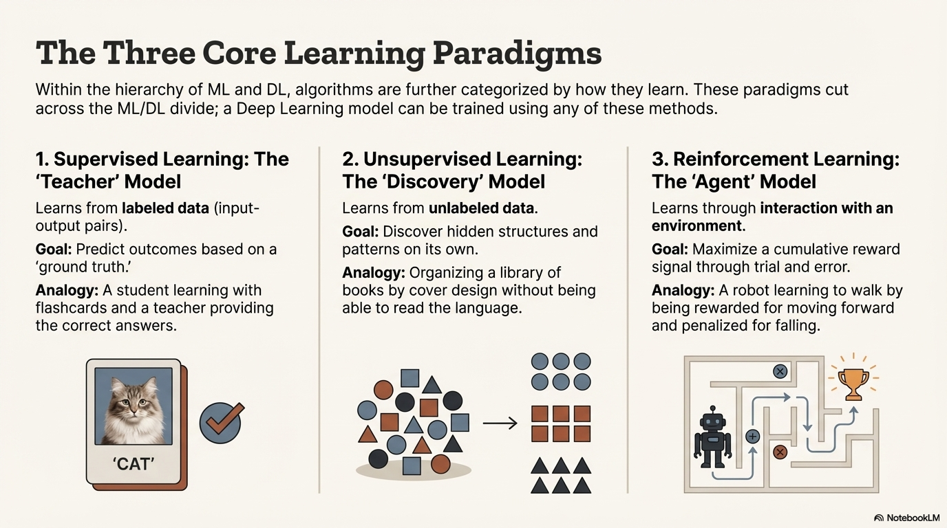
Within the broader hierarchy of ML and DL, algorithms are further categorized by how they learn. These are the three core learning paradigms: Supervised Learning, Unsupervised Learning, and Reinforcement Learning. These paradigms cut across the ML/DL divide; a Neural Network (DL) can be trained using Supervised Learning, just as a Logistic Regression model (ML) can.
5.1 Supervised Learning: The "Teacher" Model
Supervised Learning is the most prevalent paradigm in industry applications today.23 It relies on the existence of a "ground truth."
- Mechanism: The model is trained on a labeled dataset. This means every input data point is paired with the correct output label. For example, in a dataset of medical images, every X-ray is tagged by a doctor as "Normal" or "Pneumonia".13
- The Training Loop: The process is analogous to a teacher supervising a student with flashcards. The model looks at an input, makes a prediction, and compares it to the correct label. If the prediction is wrong, the system calculates the error and adjusts its internal parameters (weights) to minimize this error in the future.23
- Key Tasks:
- Classification: Predicting a discrete category. Is this email Spam or Not Spam? Is this transaction Fraudulent or Legitimate?.13
- Regression: Predicting a continuous numerical value. What will be the price of this house next year? What is the expected temperature tomorrow?.13
- Applications: Image recognition, fraud detection, spam filtering, medical diagnosis, sentiment analysis.6
5.2 Unsupervised Learning: The "Discovery" Model
Unsupervised Learning deals with unlabeled data. The system is given raw data with no instructions on what the output should be and no "answer key" to correct it.13
- Mechanism: The algorithm explores the data to find hidden structures, patterns, or groupings on its own. It effectively asks, "How is this data naturally organized?".24
- Analogy: It is like dropping a child in a massive library with books written in a language they don't speak. Even without understanding the content (labels), the child can organize the books by color, size, or symbol patterns. The child discovers the structure of the library without being told what the categories are.23
- Key Tasks:
- Clustering: Grouping similar data points together. A classic example is Customer Segmentation in marketing. An algorithm might analyze purchasing data and discover that there is a distinct group of customers who buy diapers and beer on Fridays, even if the marketing team never defined that category beforehand.13
- Dimensionality Reduction: Reducing the number of variables in a dataset while retaining essential information. Techniques like Principal Component Analysis (PCA) compress data, making it easier to visualize and process.14
- Association: Discovering rules that describe large portions of data, often used in market basket analysis (e.g., "People who buy X also buy Y").12
- Applications: Anomaly detection (cybersecurity), recommendation engines (cold-start grouping), exploratory data analysis, genomic sequencing.27
5.3 Reinforcement Learning (RL): The "Agent" Model
Reinforcement Learning differs fundamentally from the other two. It is not about analyzing a static dataset but about making a sequence of decisions in a dynamic environment.13
- Mechanism: An agent interacts with an environment. For every action the agent takes, it receives feedback in the form of a reward or a penalty.23 The agent's goal is not to be "correct" on a single prediction, but to maximize the cumulative reward over time.
- Trial and Error: The agent learns through trial and error. It might try random actions (exploration) to see what happens, and then repeat actions that yielded high rewards (exploitation). Unlike supervised learning, the feedback is often delayed—a move in a chess game might not be rewarded until the game is won 50 moves later.28
- No Labels: There is no labeled data telling the agent "this was the best move." It only knows if the outcome was positive or negative relative to its goal.25
- Applications:
- Robotics: A robot learning to walk. It receives a positive reward for moving forward and a negative penalty for falling over. Over millions of attempts, it learns the physics of walking.
- Game Playing: AlphaGo, the AI that defeated the world champion at Go, learned by playing millions of games against itself, refining its strategy based on wins and losses.23
- Autonomous Vehicles: Navigation decisions in dynamic traffic, where the "reward" is reaching the destination safely and efficiently.26
Table 1: Comparative Matrix of Learning Paradigms
| Feature | Supervised Learning | Unsupervised Learning | Reinforcement Learning |
| Data Type | Labeled Data (Input-Output pairs) | Unlabeled Data (Raw inputs) | No Predefined Data (Interaction-based) |
| Primary Goal | Predict outcomes/classes | Discover patterns/structures | Maximize cumulative reward |
| Feedback Mechanism | Direct feedback (Error minimization) | No external feedback (Self-organization) | Delayed feedback (Reward/Penalty signal) |
| Common Tasks | Classification, Regression | Clustering, Dimensionality Reduction | Navigation, Game Playing, Real-time decisions |
| Example | Predicting house prices based on historical sales | Segmenting customers by purchasing behavior | Training a chess engine by playing games |
| Human Supervision | High (Labeling required) | Low (Data prep only) | None (Agent learns autonomously) |
| Source Ref |
6. Comparative Analysis: Strategic Implementation
While DL is a subset of ML, the practical distinctions between applying "traditional ML" and "Deep Learning" are profound. Understanding these trade-offs is essential for selecting the correct approach for a given problem. It is not simply a case of "newer is better"; often, the simpler traditional ML approach is superior for specific constraints.
6.1 The Trade-off Matrix
| Criterion | Traditional Machine Learning | Deep Learning |
| Feature Engineering | Manual: Requires domain experts to identify and create features. Limits scalability but allows for human oversight. | Automatic: The network learns features directly from data. Enables handling of unstructured data but removes human control. |
| Data Dependencies | Performs well with small to mediumdatasets. Can be effective with hundreds or thousands of records. | Requires large datasets to avoid overfitting and learn representations. Typically needs tens of thousands to millions of records. |
| Hardware | Can run on standard CPUs. Low computational cost makes it viable for embedded systems. | Requires high-performance GPUs/TPUs. High computational cost requires cloud infrastructure or specialized hardware. |
| Training Time | Short (Seconds to Hours). Allows for rapid experimentation and retraining. | Long (Hours to Weeks). Retraining is expensive and time-consuming. |
| Interpretability | High: Rules are often visible (e.g., Decision Trees). Easier to audit and explain to stakeholders. | Low: "Black Box" nature makes debugging and auditing difficult. |
| Performance | Plateaus as data volume increases. Adding more data beyond a certain point yields diminishing returns. | Continues to improve as data volume increases. Follows a scaling law where more data leads to better performance. |
| Best Use Cases | Structured data (tables), simple classification, resource-constrained environments, regulated industries. | Unstructured data (images, audio, text), complex pattern recognition, generative tasks. |
6.2 The "Data-Performance" Curve
A critical insight from the research is the relationship between data volume and performance. Traditional ML algorithms tend to reach a performance plateau relatively quickly. Because they rely on a finite set of hand-engineered features, they cannot extract more nuance from the data once those features are saturated. Adding more data yields diminishing returns because the model is limited by the expressiveness of the manual features.8
Deep Learning, conversely, follows a different scaling law. Because it learns its own features, it can continue to refine its internal representations as it sees more data. It can detect subtler and subtler patterns that a human engineer might miss. This is why DL has become dominant in the era of "Big Data"—it is the only technology capable of leveraging the massive repositories of information generated by the modern internet to continuously improve performance.8
6.3 The "Black Box" Dilemma and Explainability
The shift from ML to DL represents a trade-off between Accuracy and Explainability. In regulated industries like finance or healthcare, the "Black Box" nature of DL is a significant hurdle. If a DL model denies a loan, it cannot easily explain why in human terms. It might be due to a complex, non-linear interaction between thousands of variables that has no simple linguistic description. In contrast, a Decision Tree (traditional ML) can provide a clear audit trail: "Denied because debt-to-income ratio > 40%." This has led to a resurgence of interest in "Explainable AI" (XAI) or hybrid approaches that attempt to map the opaque decisions of deep networks back to understandable features.5
7. Synthesized Conclusion
The relationship between Machine Learning, Deep Learning, and Neural Networks is not one of competition, but of evolution and specialization within the broader field of Artificial Intelligence.
The hierarchy is absolute: Deep Learning is a subset of Machine Learning, which is a subset of AI. This "Matryoshka doll" structure informs the capabilities and constraints of each layer. The defining technical fissure between traditional ML and DL is the handling of features. Traditional ML relies on human expertise to tell the computer what to look for (Feature Engineering), making it efficient but limited by human knowledge. Deep Learning relies on architecture (Neural Networks) to discover what to look for (Representation Learning), making it data-hungry and opaque but incredibly powerful for unstructured tasks.
Furthermore, the "Deep" in Deep Learning is defined by the depth of its neural networks—specifically, the use of more than three layers to facilitate hierarchical abstraction. This architecture enables the processing of complex data structures like images and language that were previously opaque to computers. Regardless of the architecture, all these systems are trained using one of the three core paradigms: Supervised (learning from examples), Unsupervised (discovering patterns), or Reinforcement (learning from interaction).
In the broader AI system, these technologies fulfill distinct roles. Traditional ML remains the workhorse for structured data analytics, business intelligence, and scenarios where interpretability is paramount. Deep Learning serves as the sensory cortex of AI, powering vision, speech, and natural language understanding. Neural Networks provide the fundamental mathematical substrate that makes this high-level cognition possible. Together, they form the composite intelligence that defines the modern algorithmic era.